PivotTables are one of Excel’s most powerful features – if not THE most powerful feature – and are exceptionally useful at summarizing large volumes of data when preparing analytical reports. But in some circumstances, you might need to summarize data to create an analytical report and a PivotTable may not be the ideal tool for that application. In that situation, you should consider using Excel’s SUMIFS function as an alternative and in this tip, you will learn how to take advantage of SUMIFS to create analytical reports.
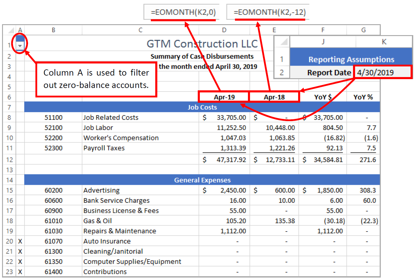
In this example, a comparative year-over-year cash disbursements report is built using the SUMIFS function on data stored in a table in the workbook; that report is pictured in Figure 1. More specifically the following formula resides in cell D15 and has been copied to other cells in columns D and E, as appropriate:
=SUMIFS(Checks[Debit],Checks[Account No],$B15,Checks[EOMONTH],D$6)
The formula above is used to identify all the transactions from the Checks table where the data in the Account No field matches the value in cell B15 (currently 60200) and also where the data in the EOMONTH field of the Checks table matches the value in cell D6 (currently 4/30/2019). When both these conditions are met, the value from the Debit column of the Checks tables is summed along with all other values from the Debit column of the Checks table for which the same criteria are met. In this fashion, the SUMIFS formula is used to create a cross-tabular report, very similar to the results generated via a PivotTable.
A few additional items of interest in this report include:
- To add end-user interaction, cell K2 uses List validation with EOMDates (a defined name) as the source of the list values.
- The formulas in cells D6 and E6 use the EOMONTH function to head the columns with the appropriate month ending dates, which are formatted with a custom date format, “mmm yyyy“.
- The formula in the YoY % column employs the IFERROR function to prevent #DIV/0 errors in those cases where the budget is equal to zero.
- The formulas in cells A8:A42 allow users to filter out accounts with zero balances. If the account balances for the current month and the same month last year are equal to zero, the formula places an “X” in the cell, which can then be filtered out of the report prior to printing.
SUMMARY
While PivotTables are often the right choice for summarizing data in Excel, in some cases a formula-based approach may be more desirable. In these situations, turning to Excel’s SUMIFS feature is often an excellent choice to generate summaries of data based on multiple conditions.