Working with Excel's CHOOSE Function
Excel’s CHOOSE function provides a great alternative to using other lookup functions when you might need to find or match data. When needing to lookup data in Excel, many business professionals instinctively turn to a formula utilizing the VLOOKUP function. In other cases, when needing to create a calculation based on a specific condition, multiple IF functions nested inside a single formula comprise the solution du jour. However, in both of these situations – and in many others – you may want to consider using Excel’s CHOOSE function as a very simple and easy-to-implement option.
Choose - The Fundamentals
At its most fundamental level, you can use CHOOSE to find the nth item in a listing of data, based on the index_num you specify in the formula. The basic syntax of a CHOOSE-based formula is as follows:
CHOOSE(index_num, value1, [value2], …)
The number of items that CHOOSE can pick from is up to 254.
To illustrate, Excel would calculate Cherries as the result of the following formula because Cherries is the third item in the list contained in the formula:
=CHOOSE(3,”Apples”,”Bananas”,”Cherries”,”Grapefruits”,”Oranges”)
Of course, if the index_num variable was “5” instead of “3,”, the formula would return a value of Oranges instead, because Oranges is the fifth item in the list.
An Example of CHOOSE in Action
Suppose you were creating a spreadsheet to calculate the amount of depreciation expense for each of the fixed assets in use in an organization. More specifically, if an asset is in the third year of its five year MACRS depreciable life, the following formula would calculate the amount of depreciation expense for the current year, assuming that cell D5 represented the depreciable basis of the asset.
=D5*CHOOSE(3,20%,32%,19.2%,11.52%,11.52%,5.76%)
Notice in this case that the index_num is a reference to a cell in the worksheet that subtracts the year of acquisition from the current year; this of course, is used to determine for which year of service should the depreciation be calculated. Assuming the depreciable basis of the asset is $1,000 and that this amount is stored in cell D5, then the above formula would return a value of $192, because 19.2% is the third item in the “lookup list.”
Like most other Excel functions, where CHOOSE really takes on power is when you combine it with other functions. Extending the previous example, the following formula takes advantage of Excel’s YEAR function to determine the appropriate rate to use when calculating depreciation for a given asset.
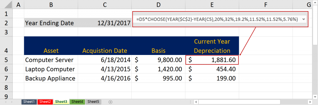
=D5*CHOOSE(YEAR($C$2)-YEAR(C5),20%,32%,19.2%,11.52%,11.52%,5.76%)
Figure 1 below shows how this formula could be used to determine the correct depreciation rate to apply to a specific asset based on the number of years the asset has been in service and then calculate the amount of depreciation expense using the CHOOSE function.
Summary
As a stand-alone function, CHOOSE provides an excellent alternative in many cases to VLOOKUP, multiple IF functions, and many other Excel functions. However, this tool really shines when you use it in tandem with other Excel functions to automate lookup tasks based on calculations. And remember, based on the index_num value in your CHOOSE functions, your formulas can return one of up to 254 alternative selections.
You can watch the video below to see how you can put CHOOSE to work to simplify many of your lookup and matching operations in Excel.
ARE YOU RECEIVING THE K2 TECH UPDATE NEWSLETTER
BY EMAIL EVERY MONTH?
Sign up now so you don’t miss the next issue.