Excel's TAKE And DROP Functions
As I’ve written repeatedly, Microsoft 365 subscribers receive new features periodically in their 365-based apps, such as Excel. Unfortunately, many users remain unaware of these features and, therefore, do not take advantage of them. To help keep you abreast of new opportunities to increase your productivity and accuracy when working with Excel, this article discusses two relatively new features available in 365-based versions of Excel – TAKE and DROP.
Simplifying Data Extractions With TAKE
Excel’s TAKE feature is a simple yet powerful function you can use to streamline copying data from one range and linking it to another. For example, suppose you have a range or table of data that extends for hundreds or even thousands of rows (or columns), but you only need to link the first five rows to another section of your workbook. You can use TAKE to accomplish this task with ease.
The syntax for TAKE is simple: =TAKE(array, rows, [columns]), where:
- Array is the range or table from which to take the data you need,
- Rows is the number of rows to take, and
- Columns is an optional argument designating the number of columns to take.
Note that if you enter a negative number for the rows argument, TAKE starts from the bottom of the range and works upward. Likewise, if you enter a negative number for the column argument, TAKE starts from the right and works to the left.
To illustrate, suppose you need to extract the top five items from the table of over 2100 rows of data pictured in Figure 1.
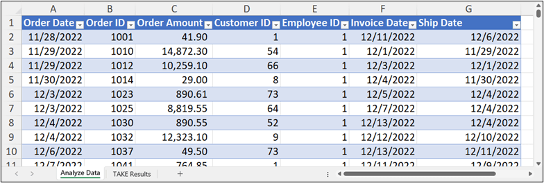
To complete the extraction, you could use the following formula that is based on Excel’s TAKE function:
=TAKE(Table1,5)
This formula extracts the first five rows from Table1, as shown in Figure 2.
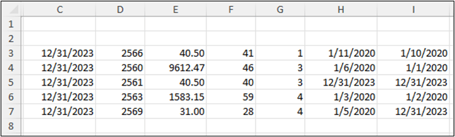
Notably, the data returned by TAKE links to the destination. Thus, if the data in the underlying data source changes, the data returned by TAKE can change, too, eliminating the need to continually copy and paste data from one location to another.
Refining Your Queries With DROP
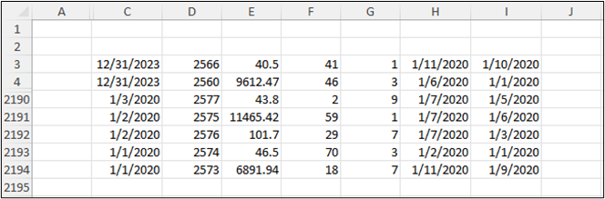
Excel’s DROP function is similar to TAKE, except that it does not return an entire array. Instead, the DROP function omits a specified number of rows or columns from the results. Thus, returning to the data in Figure 1, the following formula uses the DROP function to eliminate the header row from the formula’s results.
=DROP(Table1[#All],1)
Summary
TAKE and DROP are two relatively new functions you can use to link data from one location to another in Excel. Further, you can use these tools to refine the results so that they reflect on the data you desire to display. Accordingly, if you find that you use manual workarounds to achieve the same results, you should investigate how working with TAKE and DROP can simplify your spreadsheets.
At K2 Enterprises, our commitment lies in providing unwavering support and expert instruction to CPAs. Explore the wealth of resources on our website, where you’ll find valuable insights on selecting the most suitable accounting software, ensuring your firm is equipped with the right tools for the journey ahead. If you work in accounting or finance, K2 Enterprises provides continuing education programs to enhance your skills and credentials. Need help learning how to solve your business’s accounting technology needs and selecting the right software for accounting or CPA Firms? Visit us at k2e.com, where we make sophisticated technology understandable to anyone through our conferences, seminars, or on-demand courses.