Many consider PivotTables to be Excel’s most powerful feature, yet some Excel users struggle with formatting their PivotTable reports to exude a polished and professional appearance. If you are running Excel 2016, this process just got much easier and in this tip, you will learn how to set PivotTable options in Excel 2016 to streamline the process of formatting your PivotTables.
Newly-added for Excel 2016 is a set of PivotTable options that you can access by clicking the File tab of the Ribbon, followed by Options. Upon doing so, click Edit Default Layout as shown in Figure 1.
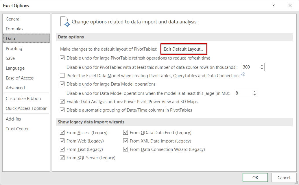 Figure 1 – Choosing to Edit the Default PivotTable Layout in Excel 2016
Next, in the Edit Default Layout dialog box pictured in Figure 2, simply establish the default layout settings you want in all new PivotTables you create. Note that these settings will show up regardless of the workbook you are in when you create new PivotTables. Further note that if an existing PivotTable already has the settings you want enabled on all future PivotTables, you only need to click in the Layout Import field and then select any cell in the PivotTable that you would like to use to establish default settings. Upon doing so, click Import and Excel will import those settings and create the default settings from them.
Figure 1 – Choosing to Edit the Default PivotTable Layout in Excel 2016
Next, in the Edit Default Layout dialog box pictured in Figure 2, simply establish the default layout settings you want in all new PivotTables you create. Note that these settings will show up regardless of the workbook you are in when you create new PivotTables. Further note that if an existing PivotTable already has the settings you want enabled on all future PivotTables, you only need to click in the Layout Import field and then select any cell in the PivotTable that you would like to use to establish default settings. Upon doing so, click Import and Excel will import those settings and create the default settings from them.
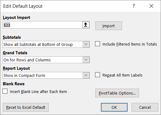 Figure 2 – PivotTable Edit Default Layout Dialog Box
Figure 1 – Choosing to Edit the Default PivotTable Layout in Excel 2016
Next, in the Edit Default Layout dialog box pictured in Figure 2, simply establish the default layout settings you want in all new PivotTables you create. Note that these settings will show up regardless of the workbook you are in when you create new PivotTables. Further note that if an existing PivotTable already has the settings you want enabled on all future PivotTables, you only need to click in the Layout Import field and then select any cell in the PivotTable that you would like to use to establish default settings. Upon doing so, click Import and Excel will import those settings and create the default settings from them.
Figure 2 – PivotTable Edit Default Layout Dialog Box